JSC 370: Data Science II

Week 9: Feature Engineering, Hyperparameter Tuning, and Model Evaluation

Outline

• Part 1: Feature Engineering
• Part 2: Hyperparameter Tuning
• Part 3: Model Evaluation — Training, Validation, and Testing
• Part 4: Cross-Validation

Where We Are

• Last week: decision trees, random forests
• We saw some hyperparameter tuning
• Showed that train/test splits let us estimate real-world performance

This week we formalize:

1. How to engineer features to improve model inputs
2. How to tune hyperparameters systematically
3. How to evaluate models honestly — split strategy and metrics

Setup

import pandas as pd
import numpy as np
import matplotlib.pyplot as plt
import requests, zipfile, io

from sklearn.model_selection import train_test_split, cross_val_score, GridSearchCV
from sklearn.tree import DecisionTreeRegressor
from sklearn.preprocessing import SplineTransformer
from xgboost import XGBRegressor, XGBClassifier
from sklearn.metrics import (accuracy_score, mean_squared_error, r2_score,
                              precision_score, recall_score, f1_score,
                              confusion_matrix, ConfusionMatrixDisplay)
import warnings
warnings.filterwarnings('ignore')

Data: Toronto Bike Share (Open Data)

We use the Toronto Open Data Bike Share Ridership dataset — individual trip records for 2023.

# Discover resources via the Toronto Open Data CKAN API
base_url = "https://ckan0.cf.opendata.inter.prod-toronto.ca"
package = requests.get(
    base_url + "/api/3/action/package_show",
    params={"id": "bike-share-toronto-ridership-data"}
).json()

Loading the 2023 Ridership Data

This is a very large dataset! We will look at May–July 2023 to capture the peak cycling season.

for r in package["result"]["resources"]:
    if "2023" in r["name"]:
        url_2023 = r["url"]
        break

# Download ZIP and read May–July (months 5–7)
resp = requests.get(url_2023)
z = zipfile.ZipFile(io.BytesIO(resp.content))

csv_files = [f for f in z.namelist() if f.endswith('.csv')][4:6]
bike = pd.concat(
    [pd.read_csv(z.open(m), encoding='latin-1') for m in csv_files],
    ignore_index=True
)
print(f"Shape: {bike.shape}")
bike.head(3)

Shape: (1252908, 10)

	Trip Id	Trip Duration	Start Station Id	Start Time	Start Station Name	End Station Id	End Time	End Station Name	Bike Id	User Type
0	21248733	344	7693	05/01/2023 00:00	NaN	7065.0	05/01/2023 00:06	Dundas St E / Parliament St	713	Annual Member
1	21248734	521	7418	05/01/2023 00:00	College Park - Yonge St Entrance	7248.0	05/01/2023 00:09	Baldwin Ave / Spadina Ave - SMART	1120	Casual Member
2	21248735	1143	7027	05/01/2023 00:01	Beverley St / Dundas St W	7279.0	05/01/2023 00:20	Rosehill Ave / Avoca Ave - SMART	2231	Casual Member

Part 1: Feature Engineering

Data preparation

We see there are several time variables and strings representing locations. Let’s start doing some data prep and cleaning for feature engineering.

bike.columns = (bike.columns
                    .str.strip()
                    .str.replace(r'\s+', '_', regex=True)
                    .str.lower())

# Parse datetime and extract temporal features
bike['start_time'] = pd.to_datetime(bike['start_time'])
bike['trip_duration_min'] = bike['trip_duration'] / 60
bike['hour']        = bike['start_time'].dt.hour
bike['day_of_week'] = bike['start_time'].dt.dayofweek   # 0=Mon, 6=Sun
bike['month']       = bike['start_time'].dt.month
bike['is_weekend']  = (bike['day_of_week'] >= 5).astype(int)
bike['is_member']   = (bike['user_type'] == 'Annual Member').astype(int)

# Keep only plausible trip durations
bike = bike[(bike['trip_duration_min'] >= 1) & (bike['trip_duration_min'] <= 120)]
print(f"Rows after filtering: {bike.shape[0]:,}")
print(f"Member rate: {bike['is_member'].mean():.1%}")
print(f"Unique start stations: {bike['start_station_id'].nunique()}")

Rows after filtering: 1,241,838
Member rate: 10.5%
Unique start stations: 675

Joining Station Geospatial Data

We also see bike station information. Station locations are published via the public GBFS feed, which is separate from the ridership data

# Fetch station info (lat, lon, capacity) from the GBFS station feed
stations = pd.DataFrame(
    requests.get(
        'https://tor.publicbikesystem.net/ube/gbfs/v1/en/station_information'
    ).json()['data']['stations']
)[['station_id', 'lat', 'lon', 'capacity']]

stations['station_id'] = stations['station_id'].astype(int)

# Join to trip data on start_station_id
bike = bike.merge(stations, left_on='start_station_id', right_on='station_id', how='left')
print(f"Stations matched: {bike['lat'].notna().sum():,} / {len(bike):,}")

Stations matched: 1,165,103 / 1,241,838

Distance from Downtown as a Feature

Raw lat/lon are correlated — distance from a reference point is often more informative

def haversine_km(lat1, lon1, lat2, lon2):
    """Great-circle distance in km between two points."""
    R = 6371
    dlat = np.radians(lat2 - lat1)
    dlon = np.radians(lon2 - lon1)
    a = (np.sin(dlat / 2) ** 2
         + np.cos(np.radians(lat1)) * np.cos(np.radians(lat2))
         * np.sin(dlon / 2) ** 2)
    return R * 2 * np.arcsin(np.sqrt(a))

# King & Bay intersection as downtown reference
DOWNTOWN_LAT, DOWNTOWN_LON = 43.6481, -79.3791
bike['dist_downtown_km'] = haversine_km(
    bike['lat'], bike['lon'], DOWNTOWN_LAT, DOWNTOWN_LON)

print(bike[['start_station_id', 'lat', 'lon',
            'capacity', 'dist_downtown_km']].head(4).round(3))

   start_station_id     lat     lon  capacity  dist_downtown_km
0              7693  43.655 -79.375      23.0             0.828
1              7418  43.660 -79.383      25.0             1.343
2              7027  43.653 -79.393      31.0             1.264
3              7027  43.653 -79.393      31.0             1.264

Summary of Toronto Bike Share Variables

Variable	Source	Type	Role
hour	start_time	Cyclical (0–23)	Predictor
day_of_week	start_time	Cyclical (0–6)	Predictor
month	start_time	Cyclical (1–12)	Predictor
is_weekend	start_time	Binary	Predictor
is_member	user_type	Binary	Predictor / Target (classification)
trip_duration_min	trip_duration	Numeric (minutes)	Target (regression)
lat, lon	GBFS station feed	Numeric	Predictor
capacity	GBFS station feed	Numeric	Predictor
dist_downtown_km	Derived from lat/lon	Numeric	Predictor
end_time	Raw data	Datetime	Beware: Leakage
end_station_id	Raw data	ID	Only known at trip end

Station Map: Duration and Member Rate

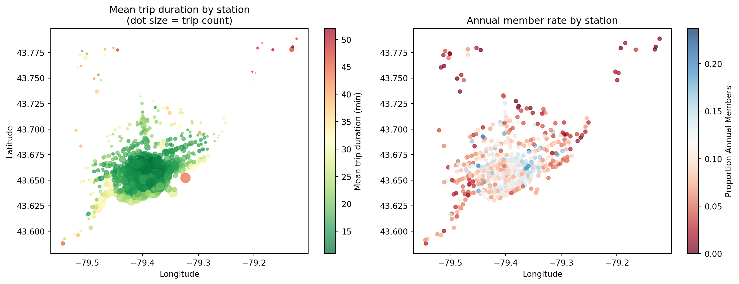
• Outer stations: longer trips, more casual users (recreational)
• Core stations: shorter trips, higher member rates (commuters)

Ridership Patterns

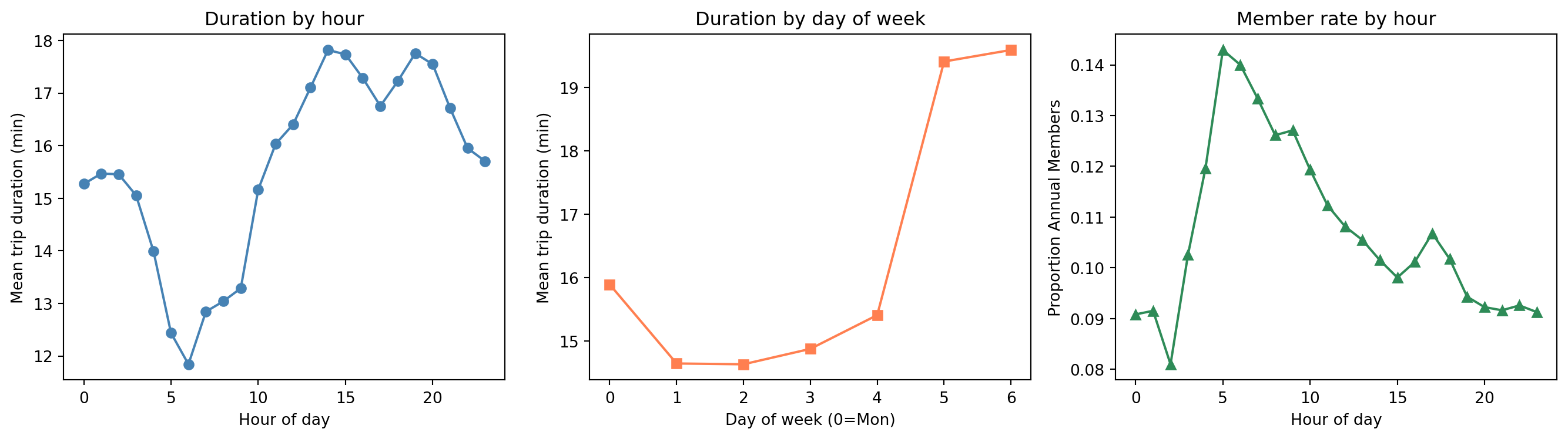
• Casual users take longer trips (recreation vs. commuting)
• Member rate spikes at commute hours (8-9am)

What is Feature Engineering?

• Feature engineering transforms raw data into inputs a model can learn from effectively
• Models only see numbers — everything must be encoded, scaled, or constructed appropriately

For the Toronto bike share data, each variable type needs different treatment:

Variable type	Example	Treatment
Cyclical	hour, day_of_week, month	Sin/cos or Fourier encoding
Binary	is_weekend, is_member	No transformation needed
Continuous numeric	dist_downtown_km, capacity	Use directly (or splines for non-linearity)
High-cardinality ID	start_station_id	Drop — replaced by spatial features

Data Leakage: Two Examples

Leakage rule: a predictor is only valid if it could be known at prediction time, before observing the outcome

Predicting trip duration

• end_time = start_time + duration → directly reveals the target
• end_station_id = only known after the trip ends

Why it matters

• Including end_time would give near-perfect R²
• But at prediction time (when trip starts) we don’t have it
• Model would fail completely in deployment

# Drop leakage columns before modelling
drop_cols = ['trip_id', 'trip_duration', 'start_time',
             'start_station_name', 'end_station_id',
             'end_time', 'end_station_name', 'bike_id', 'user_type']

The Problem with Raw Cyclical Features

• hour ranges from 0 to 23 — hour 23 and hour 0 are adjacent in time, but far apart numerically
• A linear model or distance-based model sees them as very different

Hour:  0   1   2  ...  22  23  0   1  ...
Value: 0   1   2  ...  22  23  0   1  ...  ← model sees a big jump at midnight

• The same problem affects day of week (6 → 0) and month (12 → 1)
• One-hot encoding fixes the adjacency problem but loses the ordering information (the model no longer knows that hour 5 is between hours 4 and 6)

Solution: encode cyclical variables using sine and cosine transforms

Sine-Cosine Encoding for Cyclical Features

For a variable with period \(T\) (e.g., \(T = 24\) for hours, \(T = 12\) for months):

\[\sin\!\left(\frac{2\pi \cdot x}{T}\right), \quad \cos\!\left(\frac{2\pi \cdot x}{T}\right)\]

• This maps each value onto a circle — hour 23 and hour 0 are now close together
• Two columns preserve both ordering and wrap-around

bike['hour_sin']  = np.sin(2 * np.pi * bike['hour'] / 24)
bike['hour_cos']  = np.cos(2 * np.pi * bike['hour'] / 24)
bike['dow_sin']   = np.sin(2 * np.pi * bike['day_of_week'] / 7)
bike['dow_cos']   = np.cos(2 * np.pi * bike['day_of_week'] / 7)
bike['month_sin'] = np.sin(2 * np.pi * bike['month'] / 12)
bike['month_cos'] = np.cos(2 * np.pi * bike['month'] / 12)
print(bike[['hour', 'hour_sin', 'hour_cos']].head(6).round(3))

   hour  hour_sin  hour_cos
0     0       0.0       1.0
1     0       0.0       1.0
2     0       0.0       1.0
3     0       0.0       1.0
4     0       0.0       1.0
5     0       0.0       1.0

Visualizing Cyclical Encoding of Hour

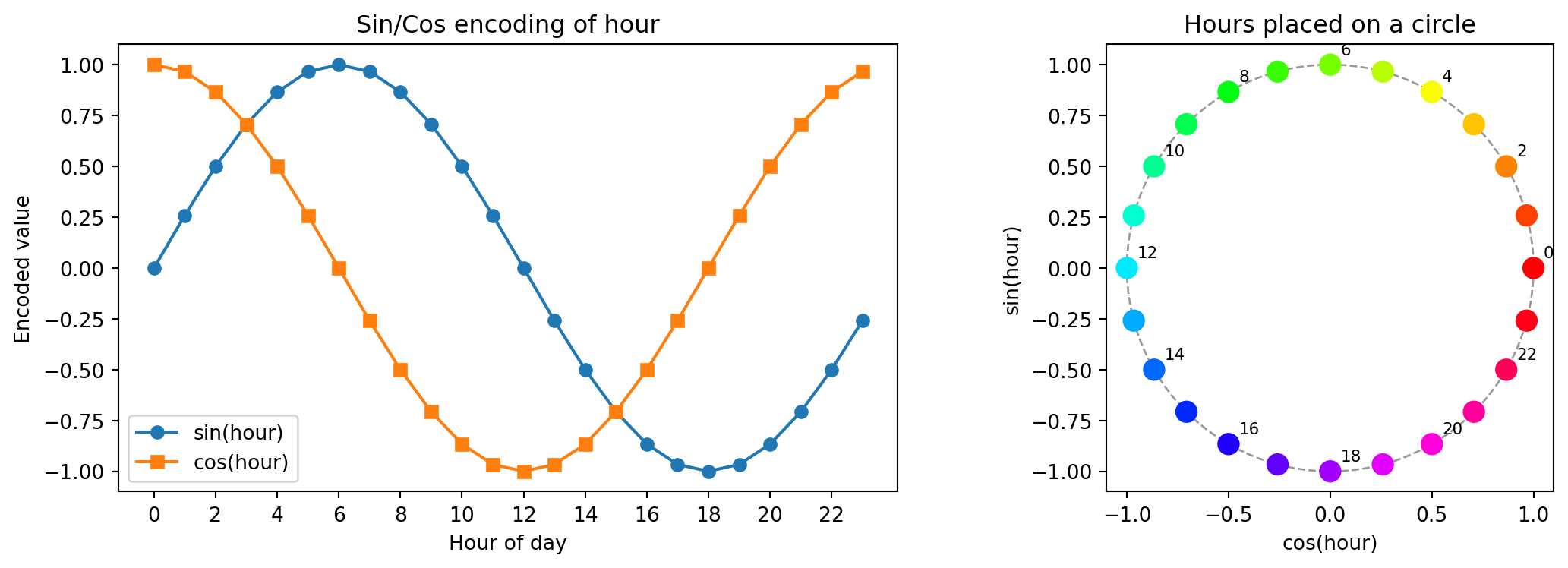
Hour 23 and hour 0 are now adjacent in the encoded space

Fourier Features for Capturing Multiple Harmonics

• A single sin/cos pair captures one frequency (one peak per cycle)
• The hourly member-rate pattern has two peaks (AM and PM commute) — one cycle per 12 hours

Add \(K\) harmonics for period \(T\):

\[\sin\!\left(\frac{2\pi k \cdot x}{T}\right), \; \cos\!\left(\frac{2\pi k \cdot x}{T}\right), \quad k = 1, 2, \dots, K\]

def fourier_features(series, period, n_harmonics, name):
    cols = {}
    for k in range(1, n_harmonics + 1):
        cols[f'{name}_sin_k{k}'] = np.sin(2 * np.pi * k * series / period)
        cols[f'{name}_cos_k{k}'] = np.cos(2 * np.pi * k * series / period)
    return pd.DataFrame(cols, index=series.index)

# 3 harmonics for hour (captures multiple peaks in the day)
hr_fourier = fourier_features(bike['hour'], period=24, n_harmonics=3, name='hr')
print(hr_fourier.head(3).round(3))

   hr_sin_k1  hr_cos_k1  hr_sin_k2  hr_cos_k2  hr_sin_k3  hr_cos_k3
0        0.0        1.0        0.0        1.0        0.0        1.0
1        0.0        1.0        0.0        1.0        0.0        1.0
2        0.0        1.0        0.0        1.0        0.0        1.0

Fourier Harmonics for the Daily Cycle

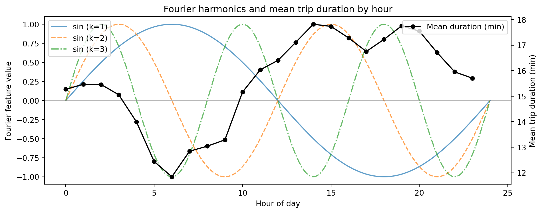
• \(k=1\): one cycle per day — misses the two-peak commute pattern
• \(k=2\): two cycles per day — captures AM/PM variation
• Higher harmonics add finer-grained structure

Splines for Smooth Non-Linear Effects

• Fourier features capture periodic patterns for known-period cyclical variables
• For general continuous predictors (e.g., temperature, humidity), use splines

We saw this earlier in the semester. Splines fit a piecewise polynomial, smooth at knot locations — flexible non-linear features

# Example: spline basis for a continuous predictor
x_vals = np.linspace(0, 1, 300).reshape(-1, 1)
spline = SplineTransformer(n_knots=5, degree=3, include_bias=False)
basis = spline.fit_transform(x_vals)
print(f"Input shape: {x_vals.shape}  →  Spline features: {basis.shape}")

Input shape: (300, 1)  →  Spline features: (300, 6)

• degree=3: cubic spline — smooth first and second derivatives at each knot
• n_knots=5 → 7 basis columns, each active in a local region
• Practical use: dist_downtown_km has a non-linear relationship with trip duration — splines can capture this; weather variables (if joined from Environment Canada) are another good candidate

Visualizing Spline Basis Functions

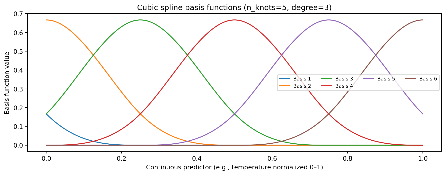
Each basis function is non-zero only locally — the model can assign different coefficients to each region

Fourier vs Splines

	Fourier features	Splines
Best for	Known periodic patterns (hour, month, day_of_week)	Smooth trends of any shape (temp, humidity)
Captures	Multiple harmonics of a fixed period	Local, flexible non-linearity
Key parameters	Period \(T\), harmonics \(K\)	Knots, degree
Extrapolation	Periodic — repeats outside training range	Can diverge outside range
Interpretability	Spectral / frequency decomposition	Piecewise polynomial

In practice, combine them:

• Fourier features for hour, day_of_week, month (known periods)
• Splines for continuous predictors like dist_downtown_km (non-linear effect on duration)
• Binary flags for is_weekend, is_member

Assembling the Full Feature Set

def build_features(df):
    out = pd.DataFrame(index=df.index)
    # Binary flags (no transformation needed)
    out['is_weekend'] = df['is_weekend']
    out['is_member']  = df['is_member']
    # Fourier features for cyclical variables
    for col, period, K in [('hour', 24, 3), ('day_of_week', 7, 2), ('month', 12, 2)]:
        for k in range(1, K + 1):
            out[f'{col}_sin_k{k}'] = np.sin(2 * np.pi * k * df[col] / period)
            out[f'{col}_cos_k{k}'] = np.cos(2 * np.pi * k * df[col] / period)
    # Spatial features from GBFS station join
    out['dist_downtown_km'] = df['dist_downtown_km']
    out['capacity']         = df['capacity']
    return out

X     = build_features(bike)
X_cls = X.drop(columns=['is_member'])  # is_member is the target for classification
y_reg = bike['trip_duration_min']      # regression target
y_cls = bike['is_member']              # classification target

print(f"Regression features:     {X.shape[1]}")
print(f"Classification features: {X_cls.shape[1]}")

Regression features:     18
Classification features: 17

Feature Importance: How It’s Calculated in XGBoost

Every time a tree splits on feature \(j\), the reduction in impurity is recorded:

\[\Delta I_j = I(\text{parent}) - \frac{n_L}{n} I(\text{left}) - \frac{n_R}{n} I(\text{right})\]

• For regression: impurity = MSE → each split reduces prediction error
• For classification: impurity = Gini or entropy → each split improves class separation
• Feature importance = weighted average of \(\Delta I_j\) across all splits and all trees that used feature \(j\)

xgb = XGBRegressor(importance_type='gain')   # 'gain', 'weight', or 'cover'
xgb.fit(X_train, y_train)
xgb.feature_importances_   # array of length n_features, sums to 1

importance_type	Meaning
'gain'	Average reduction in loss when feature is used (closest to MDI)
'weight'	Number of times feature appears in splits (default)
'cover'	Average number of samples covered by splits on this feature

Fitting Models for Both Tasks

X_train,   X_test,   y_train,   y_test   = train_test_split(
    X,     y_reg, test_size=0.3, random_state=65)
X_train_c, X_test_c, y_train_c, y_test_c = train_test_split(
    X_cls, y_cls, test_size=0.3, random_state=65)

# Regression: predict trip duration (X includes is_member as a predictor)
xgb_reg = XGBRegressor(n_estimators=200, max_depth=5, learning_rate=0.1,
                        importance_type='gain', random_state=65, n_jobs=-1)
xgb_reg.fit(X_train, y_train)

# Classification: predict annual member vs casual (X_cls excludes is_member)
xgb_cls = XGBClassifier(n_estimators=200, max_depth=5, learning_rate=0.1,
                         importance_type='gain', random_state=65, n_jobs=-1)
xgb_cls.fit(X_train_c, y_train_c)

imp_reg = pd.Series(xgb_reg.feature_importances_, index=X.columns)
imp_cls = pd.Series(xgb_cls.feature_importances_, index=X_cls.columns)

# Test metrics — regression
y_pred_reg = xgb_reg.predict(X_test)
rmse = np.sqrt(mean_squared_error(y_test, y_pred_reg))
r2   = r2_score(y_test, y_pred_reg)
print(f"Regression     — RMSE: {rmse:.2f} min  | R²: {r2:.4f}")

# Test metrics — classification
y_pred_cls = xgb_cls.predict(X_test_c)
acc = accuracy_score(y_test_c, y_pred_cls)
f1  = f1_score(y_test_c, y_pred_cls)
print(f"Classification — Accuracy: {acc:.4f}  | F1: {f1:.4f}")

print("\nTop 3 (regression):", imp_reg.nlargest(3).round(3).to_dict())
print("Top 3 (classification):", imp_cls.nlargest(3).round(3).to_dict())

Regression     — RMSE: 13.49 min  | R²: 0.1354
Classification — Accuracy: 0.8946  | F1: 0.0000

Top 3 (regression): {'is_weekend': 0.3720000088214874, 'is_member': 0.17399999499320984, 'dist_downtown_km': 0.13899999856948853}
Top 3 (classification): {'month_sin_k1': 0.7540000081062317, 'is_weekend': 0.057999998331069946, 'hour_sin_k1': 0.029999999329447746}

Feature Importance: Regression vs Classification

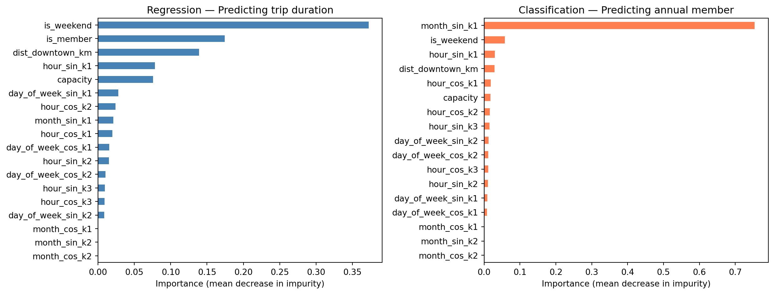
What the Importances Tell Us

Predicting trip duration (uses X, includes is_member)

• is_weekend — longer leisure rides on weekends
• is_member — casual users tend to ride longer; likely the strongest predictor
• dist_downtown_km — outer stations generate longer trips
• Hour-of-day harmonics — commuter vs. leisure timing

Predicting annual member (uses X_cls, is_member excluded)

• month and hour Fourier features — commute-month patterns strongly distinguish members
• is_weekend — casual users dominate weekends
• dist_downtown_km — station distance from downtown
• capacity — larger hubs skew toward members

However, the model performance is not great for either!

Part 2: Hyperparameter Tuning

Parameters vs Hyperparameters

	Parameters	Hyperparameters
What	Learned from data	Set before training
Examples (XGBoost)	Tree split values, leaf weights	n_estimators, max_depth, learning_rate
How chosen	Optimization (minimize loss)	Search + validation

• Parameters are what the model learns during fit()
• Hyperparameters control how the learning happens — not updated by optimization

XGBoost Regularized Objective

At each boosting round, XGBoost minimizes a penalized loss:

\[\mathcal{L} = \sum_i \ell(y_i, \hat{y}_i) + \sum_k \left[ \gamma T_k + \frac{1}{2}\lambda \|w_k\|^2 + \alpha \|w_k\|_1 \right]\]

Parameter	Role	Effect	Default
reg_lambda \((\lambda)\)	L2 on leaf weights	Smooth shrinkage toward zero; reduces variance	1
reg_alpha \((\alpha)\)	L1 on leaf weights	Drives small weights to exactly zero; sparsity	0
gamma \((\gamma)\)	Min gain to split	Prunes splits that don’t reduce loss enough	0

• L2 (reg_lambda) is on by default — partly why XGBoost generalizes well out of the box
• L1 (reg_alpha) is useful when many features are present and only a few are expected to matter
• gamma is a complementary handle on tree complexity alongside max_depth

The Bias-Variance Tradeoff

\[\text{Expected Test Error} = \text{Bias}^2 + \text{Variance} + \text{Irreducible Error}\]

• Bias: error from wrong assumptions — model too simple to capture the true pattern
• Variance: error from sensitivity to training data — model fits noise
• Irreducible error: noise in the data — no model can eliminate this

Hyperparameter tuning searches for the model complexity that minimizes test error

Bias-Variance: Boosting Rounds vs RMSE

Unlike a single tree, XGBoost adds trees sequentially — more rounds can overfit

xgb_bv = XGBRegressor(n_estimators=600, max_depth=5, learning_rate=0.1,
                       random_state=65, n_jobs=-1)
xgb_bv.fit(X_train, y_train)

n_rounds = list(range(10, 610, 10))
train_err, test_err = [], []
for n in n_rounds:
    tr = xgb_bv.predict(X_train, iteration_range=(0, n))
    te = xgb_bv.predict(X_test,  iteration_range=(0, n))
    train_err.append(np.sqrt(mean_squared_error(y_train, tr)))
    test_err.append(np.sqrt(mean_squared_error(y_test,  te)))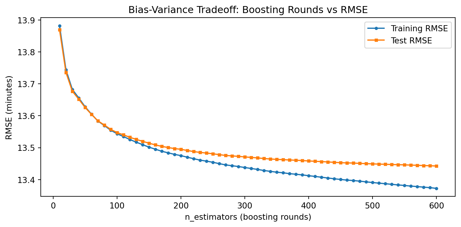

• Few rounds: high bias (underfitting)
• Too many rounds: training error keeps falling, test error rises (overfitting)
• Early stopping can automatically find the sweet spot

Hyperparameter Tuning with Cross-Validation

XGBoost has no OOB score — use 5-fold CV with random search when the grid is large

from sklearn.model_selection import RandomizedSearchCV

param_dist = {
    'max_depth':     [3, 5, 7],
    'learning_rate': [0.05, 0.1, 0.3],
    'reg_lambda':    [0.1, 1, 10],   # L2: smooth shrinkage
    'reg_alpha':     [0, 0.1, 1],    # L1: sparsity on leaf weights
}
xgb = XGBRegressor(n_estimators=250, random_state=65, n_jobs=-1)
rand_search = RandomizedSearchCV(xgb, param_dist, n_iter=20, cv=5,
                                 scoring='neg_root_mean_squared_error',
                                 random_state=65, n_jobs=-1)
rand_search.fit(X_train, y_train)
print("Best params:", rand_search.best_params_)
print(f"Best CV RMSE: {-rand_search.best_score_:.2f} minutes")

• Full grid: \(3^4 = 81\) combinations × 5 folds = 405 fits — slow on large datasets
• Random search samples 20 random combinations × 5 folds = 100 fits — much faster
• For small datasets or few hyperparameters, GridSearchCV is fine and exhaustive
• Best params: {‘reg_lambda’: 10, ‘reg_alpha’: 0.1, ‘max_depth’: 7, ‘learning_rate’: 0.3}

Fit the Best Model

#best_params = rand_search.best_params_
#print("Best params:", best_params)

xgb_best = XGBRegressor(
    n_estimators=250,
    reg_lambda=10, reg_alpha=0.1, max_depth=7, learning_rate=0.3,
    random_state=65, n_jobs=-1
)
xgb_best.fit(X_train, y_train)
y_pred = xgb_best.predict(X_test)

print(f"Test RMSE: {np.sqrt(mean_squared_error(y_test, y_pred)):.2f} minutes")
print(f"Test R²:   {r2_score(y_test, y_pred):.4f}")

Test RMSE: 13.41 minutes
Test R²:   0.1466

Early Stopping: Automatic Tuning of n_estimators

XGBoost can automatically stop adding trees when validation error stops improving

X_tr, X_val, y_tr, y_val = train_test_split(
    X_train, y_train, test_size=0.2, random_state=65)

xgb_es = XGBRegressor(
    n_estimators=2000, max_depth=5, learning_rate=0.05,
    early_stopping_rounds=50, random_state=65, n_jobs=-1
)
xgb_es.fit(X_tr, y_tr,
           eval_set=[(X_val, y_val)],
           verbose=False)
print(f"Best round: {xgb_es.best_iteration}")
print(f"Val RMSE:   {xgb_es.best_score:.2f} minutes")

• Set n_estimators very large; training stops after 50 rounds with no improvement
• Efficient alternative to grid-searching n_estimators separately

Tuning Strategy Summary

Method	When to use	Pros	Cons
Grid search + CV	Few hyperparameters	Exhaustive, unbiased	Expensive for large grids
Random search + CV	Many hyperparameters	Efficient, scales well	May miss optimal
Early stopping	XGBoost / LightGBM	Automatically tunes n_estimators	Needs a validation set
OOB score	Random forests only	Free — no extra fitting	RF-specific

• For XGBoost: use grid/random search for max_depth + learning_rate; use early stopping for n_estimators
• Always tune on training data — report final performance on the test set

Part 3: Model Evaluation

What Are We Predicting?

We use the Toronto Bike Share 2023 dataset throughout this lecture.

Regression task (this section):

• Target: trip_duration_min — trip duration in minutes, filtered to 1–120 min
• Features: temporal (hour, day of week, month via Fourier encoding), spatial (distance from downtown, station capacity), membership status (is_member)
• Question: How long will a trip take, given when and where it starts?

Classification task (later in this section):

• Target: is_member — annual member (1) vs. casual rider (0)
• Question: Can we identify member rides from trip characteristics alone?

The Three Roles of Data

Role	Purpose	May influence model?
Training set	Fit model parameters	Yes — model learns from this
Validation set	Tune hyperparameters, select model	Yes — guides tuning decisions
Test set	Report final performance	No — evaluated once at the end

• The test set is a lockbox — do not open it until the final model is chosen
• Using the test set to guide any decision inflates performance estimates

Train / Validation / Test Split

All data
├── Training set (60%)   → fit model parameters
├── Validation set (20%) → tune hyperparameters, select model
└── Test set (20%)       → final, unbiased evaluation (untouched until the end)

# First, hold out the test set
X_trainval, X_test, y_trainval, y_test = train_test_split(
    X, y_reg, test_size=0.2, random_state=65
)
# Then split training from validation
X_train, X_val, y_train, y_val = train_test_split(
    X_trainval, y_trainval, test_size=0.25, random_state=65
    # 0.25 × 0.8 = 0.2 of original → 60 / 20 / 20 split
)
print(f"Train: {X_train.shape[0]:,}  |  Val: {X_val.shape[0]:,}  |  Test: {X_test.shape[0]:,}")

Train: 745,102  |  Val: 248,368  |  Test: 248,368

Fitting and Evaluating on the Split

Train on X_train, use X_val to confirm the model generalises, then retrain on X_trainval (train + val) before evaluating once on X_test:

# 1. Fit on training set
model_val = XGBRegressor(n_estimators=250, reg_lambda=10, reg_alpha=0.1,
                         max_depth=7, learning_rate=0.3,
                         random_state=65, n_jobs=-1)
model_val.fit(X_train, y_train)
val_rmse = np.sqrt(mean_squared_error(y_val, model_val.predict(X_val)))
print(f"Validation RMSE: {val_rmse:.2f} min")

# 2. Retrain on train + val, then evaluate on test (open the lockbox once)
model_final = XGBRegressor(n_estimators=250, reg_lambda=10, reg_alpha=0.1,
                            max_depth=7, learning_rate=0.3,
                            random_state=65, n_jobs=-1)
model_final.fit(X_trainval, y_trainval)
y_pred = model_final.predict(X_test)
test_rmse = np.sqrt(mean_squared_error(y_test, y_pred))
print(f"Test RMSE:       {test_rmse:.2f} min")

Validation RMSE: 13.40 min
Test RMSE:       13.38 min

Regression Metrics

Metric	Formula	Interpretation
RMSE	\(\sqrt{\frac{1}{n}\sum(y_i - \hat y_i)^2}\)	Error in same units as \(y\)
MAE	\(\frac{1}{n}\sum\|y_i - \hat y_i\|\)	Average absolute error (robust to outliers)
R²	\(1 - \frac{\sum(y_i - \hat y_i)^2}{\sum(y_i - \bar y)^2}\)	Proportion of variance explained

rmse = np.sqrt(mean_squared_error(y_test, y_pred))
mae  = np.mean(np.abs(y_test - y_pred))
r2   = r2_score(y_test, y_pred)
print(f"RMSE: {rmse:.1f} minutes")
print(f"MAE:  {mae:.1f} minutes")
print(f"R²:   {r2:.4f}")

RMSE: 13.4 minutes
MAE:  8.8 minutes
R²:   0.1479

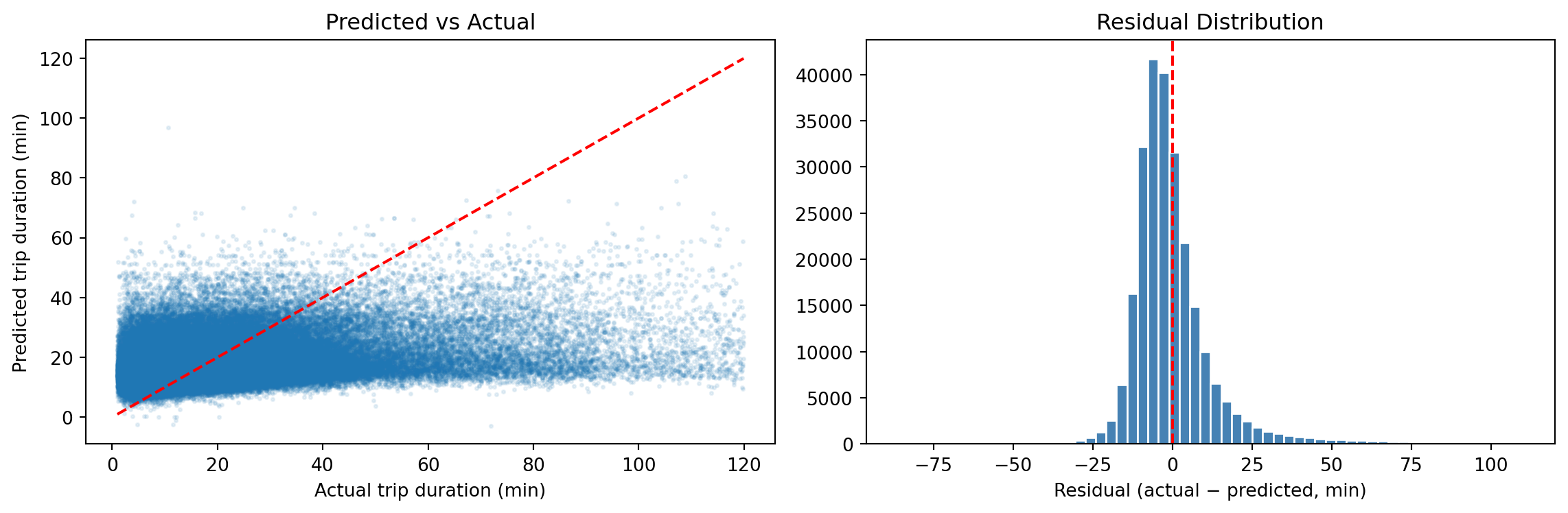
Residual Plot

Classification: Predicting Annual Member vs Casual

We can also predict user type — whether a rider is an annual member or a casual user

X_train_c, X_test_c, y_train_c, y_test_c = train_test_split(
    X_cls, y_cls, test_size=0.3, random_state=65)  # X_cls excludes is_member

# Class imbalance: members are the majority class
n_casual  = (y_train_c == 0).sum()
n_member  = (y_train_c == 1).sum()
spw = n_casual / n_member
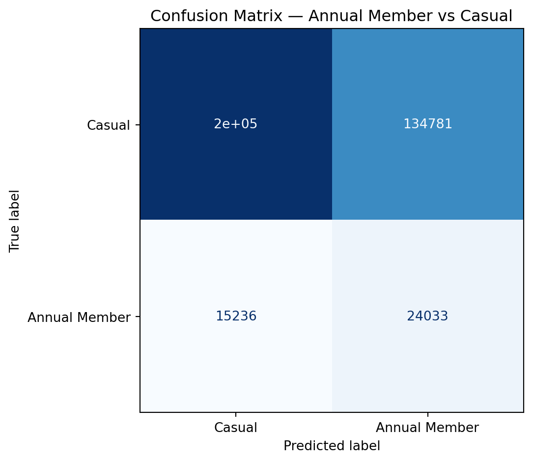
print(f"Casual: {n_casual:,}  |  Member: {n_member:,}  |  scale_pos_weight: {spw:.2f}")

Casual: 777,807  |  Member: 91,479  |  scale_pos_weight: 8.50

If the data has ~65% members, a naive model can achieve 65% accuracy by predicting “member” every time — accuracy alone is misleading. scale_pos_weight re-weights the loss so each class contributes equally:

\[\texttt{scale_pos_weight} = \frac{n_{\text{casual}}}{n_{\text{member}}}\]

clf = XGBClassifier(n_estimators=200, max_depth=5, learning_rate=0.1,
                    scale_pos_weight=spw,
                    random_state=65, n_jobs=-1)
clf.fit(X_train_c, y_train_c)
y_pred_cls = clf.predict(X_test_c)

print(f"Accuracy:  {accuracy_score(y_test_c, y_pred_cls):.4f}")
print(f"Precision: {precision_score(y_test_c, y_pred_cls):.4f}")
print(f"Recall:    {recall_score(y_test_c, y_pred_cls):.4f}")
print(f"F1:        {f1_score(y_test_c, y_pred_cls):.4f}")

Accuracy:  0.5973
Precision: 0.1513
Recall:    0.6120
F1:        0.2427

Classification Metrics Explained

	Predicted Member	Predicted Casual
Actual Member	TP (true positive)	FN (false negative)
Actual Casual	FP (false positive)	TN (true negative)

\[\text{Precision} = \frac{TP}{TP + FP} \qquad \text{Recall} = \frac{TP}{TP + FN} \qquad F1 = \frac{2 \cdot P \cdot R}{P + R}\]

• High precision, low recall: model is conservative — rarely predicts “Member” but usually correct when it does
• High recall, low precision: catches most members but many false alarms
• F1: harmonic mean — balances precision and recall

Confusion Matrix

Choosing the Right Metric

Scenario	Recommended metric
Balanced classification	Accuracy or F1
Imbalanced classification (rare event)	Precision, Recall, F1, AUC-ROC
Regression, large errors costly	RMSE
Regression, outliers present	MAE
Regression, explain variance	R²

• Choose your metric before looking at results — changing metrics after seeing performance is a subtle form of overfitting

Part 4: Cross-Validation

The Problem with a Single Validation Set

• A single train/validation split introduces high variance in the performance estimate
• Results depend heavily on which observations end up in each set

Split 1: val = [obs 1, 5, 9, ...]   → RMSE = 8.4 min
Split 2: val = [obs 2, 6, 10, ...]  → RMSE = 7.9 min
Split 3: val = [obs 3, 7, 11, ...]  → RMSE = 8.8 min

Cross-validation averages over many splits to reduce this variance

\(k\)-Fold Cross-Validation

Data: [Fold 1] [Fold 2] [Fold 3] [Fold 4] [Fold 5]

Iter 1: TRAIN   TRAIN   TRAIN   TRAIN   [VAL  ]  → score₁
Iter 2: TRAIN   TRAIN   TRAIN   [VAL  ] TRAIN    → score₂
Iter 3: TRAIN   TRAIN   [VAL  ] TRAIN   TRAIN    → score₃
Iter 4: TRAIN   [VAL  ] TRAIN   TRAIN   TRAIN    → score₄
Iter 5: [VAL  ] TRAIN   TRAIN   TRAIN   TRAIN    → score₅

CV score = mean(score₁, …, score₅)

• Every observation is used for both training and validation — just never at the same time
• Common choices: \(k = 5\) or \(k = 10\)
• Test set remains held out throughout

Cross-Validation in Python

xgb_cv = XGBRegressor(n_estimators=250, max_depth=5, learning_rate=0.1,
                       random_state=65, n_jobs=-1)
cv_scores = cross_val_score(xgb_cv, X_train, y_train, cv=5,
                             scoring='neg_root_mean_squared_error')
print(f"5-fold CV RMSE: {-cv_scores.mean():.2f} ± {cv_scores.std():.2f} minutes")
print(f"Individual folds: {(-cv_scores).round(2)}")

5-fold CV RMSE: 13.52 ± 0.04 minutes
Individual folds: [13.5  13.5  13.47 13.51 13.6 ]

# Final test evaluation
xgb_cv.fit(X_train, y_train)
test_rmse = np.sqrt(mean_squared_error(y_test, xgb_cv.predict(X_test)))
print(f"Test RMSE: {test_rmse:.2f} minutes")

Test RMSE: 13.47 minutes

Leave-One-Out Cross-Validation (LOOCV)

• Extreme case of \(k\)-fold with \(k = n\): each fold contains a single observation
• Train on \(n - 1\) observations, validate on 1

\[\text{LOOCV Error} = \frac{1}{n} \sum_{i=1}^n \text{Error}_i\]

	LOOCV	5-fold CV
Bias	Very low (model sees nearly all data)	Slightly higher
Variance	High (single observation in each val set)	Lower
Computation	\(n\) model fits	5 model fits
When to use	Very small datasets only	Standard recommendation

In practice, 5- or 10-fold CV gives a better bias-variance tradeoff than LOOCV However, in bocked data settings, such as spatial and temporal data we sometimes do leave one site out (LOSO) or leave one time period out (LOTO) cross validation rather than LOOCV

Data Leakage and the Feature Engineering Pipeline

A correct workflow applies all transformations inside the train/test split:

# Wrong: fit scaler on full data (leaks test info into training)
scaler.fit(X)   # test statistics contaminate training

# Right: fit only on training data
scaler.fit(X_train)
X_train_scaled = scaler.transform(X_train)
X_test_scaled  = scaler.transform(X_test)  # apply fitted scaler to test

scikit-learn Pipelines bundle preprocessing + model so that CV applies them correctly:

from sklearn.pipeline import Pipeline
pipe = Pipeline([
    ('spline', SplineTransformer(n_knots=5, degree=3)),
    ('model',  XGBRegressor(n_estimators=200, max_depth=5, random_state=65))
])
# Spline is fit only on training fold — no leakage
cv_pipe = cross_val_score(pipe, X_train[['hour']], y_train, cv=5,
                           scoring='neg_root_mean_squared_error')
print(f"CV RMSE with spline: {-cv_pipe.mean():.2f} minutes")

The Full ML Workflow

1. Understand the data — identify leakage variables (end_time, end_station_id)

2. Split data → train (70%) / test (30%)

3. Feature engineering (on training data only)

   • Fourier features for hour, day_of_week, month
   • Binary flags for is_weekend, is_member
   • Spatial features: dist_downtown_km, capacity (from GBFS station join)
   • (Optional: splines for dist_downtown_km; weather if joined from Environment Canada)

4. Hyperparameter tuning (5-fold CV on training data only)

   • Grid search over max_depth in [3, 5, 7] and learning_rate in [0.05, 0.1, 0.3]
   • Early stopping to find optimal n_estimators

5. Refit final model on full training set with best hyperparameters

6. Evaluate on test set (once)

   • Regression (trip duration): RMSE, MAE, R²
   • Classification (member type): accuracy, F1, confusion matrix

7. Interpret results — feature importance, residual plots

Summary

Feature Engineering

• Encode cyclicals with sin/cos or Fourier features (hour, day_of_week, month)
• Drop leakage variables (end_time, end_station_id) before modelling
• Use splines for smooth non-linear effects of continuous predictors (e.g., temperature)
• Always fit transformers on training data only

Hyperparameter Tuning

• Grid or random search + 5-fold CV on training data only; use random search when the grid is large
• Key XGBoost parameters:

Parameter	Role	Default
max_depth	Tree complexity	6
learning_rate	Shrinkage per boosting step	0.3
n_estimators	Number of boosting rounds	100
reg_lambda	L2 penalty on leaf weights — reduces variance	1
reg_alpha	L1 penalty on leaf weights — encourages sparsity	0
gamma	Min loss reduction required to make a split	0

• Use early stopping to efficiently tune n_estimators; use random search for the rest

Model Evaluation

• Test set reveals true generalization — use it once
• Use CV on training data for tuning and model selection
• RMSE/R² for regression; F1/AUC for classification